Bioinformatics Laboratory at BiUH.
Core Values: Respect, Reflection, Communication, Commitment.
Loading......
Password
Section 1. Function Fundamentals
What is a Function?
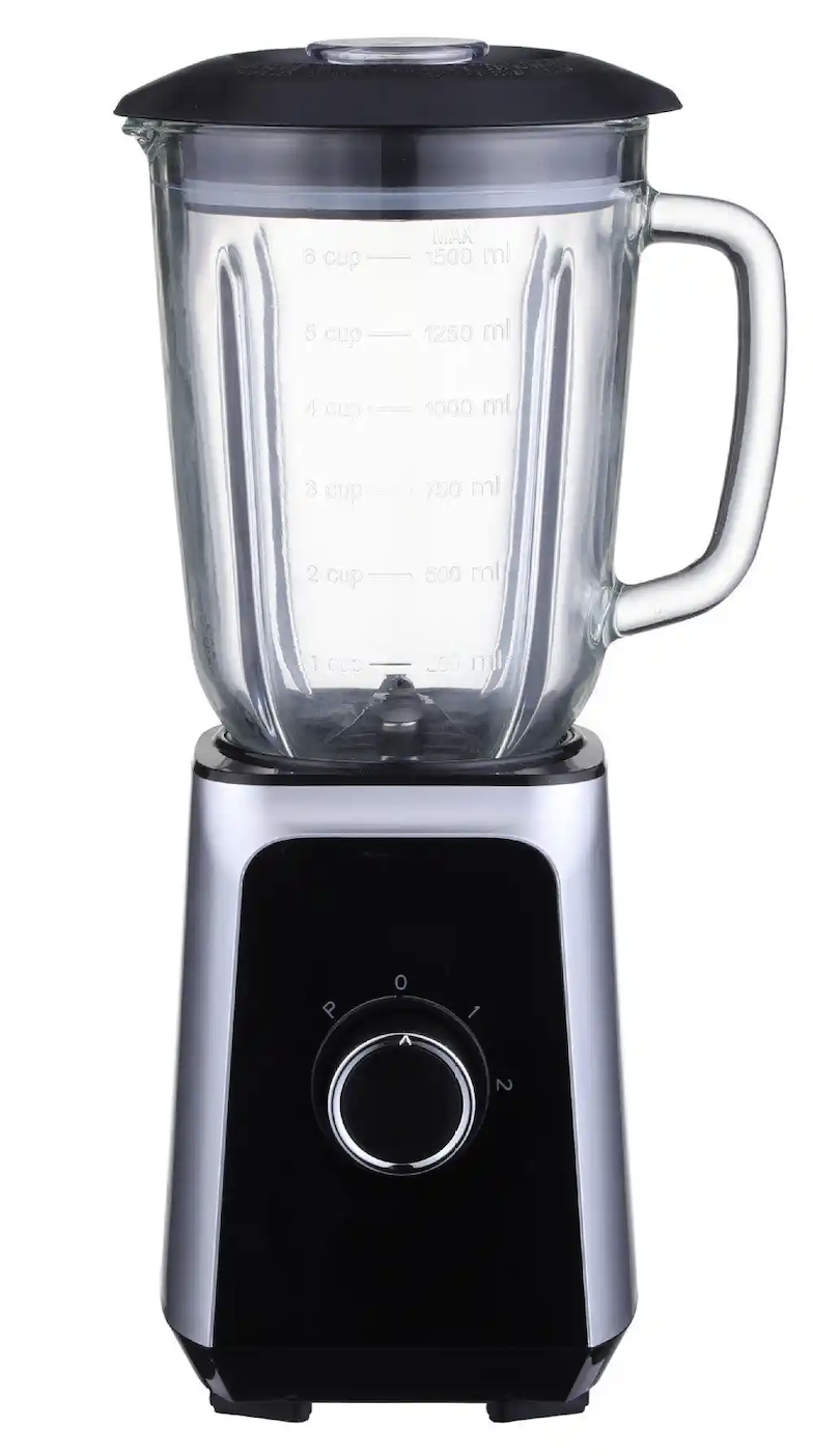
Like a juicer machine:
- Input: Whole fruits (arguments)
- Processing: Juicing mechanism (function body)
- Output: Fresh juice (return value)


Ready-made Functions: sum()
# Calculate total score
math_scores <- c(75, 88, 92, 65)
sum(math_scores)

# [1] 320
Ready-made Functions: mean()
# Find average score
mean(math_scores)
# [1] 80

# add element into a vector
c(math_scores, NA)
What if we add NA value?
mean(c(math_scores, NA)) ➔ NA
mean(c(math_scores, NA), na.rm = TRUE) ➔ ??
Ready-made Functions: paste()
# Combine text
students <- c("Alice", "Bob", "Charlie")
paste(students, "got", math_scores)

# [1] "Alice got 75"   "Bob got 88"     "Charlie got 92"
Create Your First Function
c_to_f <- function(celsius) {
    fahrenheit <- celsius * 9/5 + 32
    return(fahrenheit)
   }

# function name: c_to_f
# claim a function: function
# parameter: celsius
# function body: curly braces {}
# return value: return()

# Test it!
c_to_f(0)   # 32°F (freezing point)
c_to_f(100) # 212°F (boiling point)
Question: f_to_c ?
convert a temperature from fahrenheit to celsius
Question: can you add some “print()” to describe the function of this function and the output of this function
Qustion: what kind of error will we meet?
Function Parameters: BMI Calculator
Calculate Body Mass Index
calculate_bmi <- function(weight_kg, height_m=1.7) {
    bmi <- weight_kg / (height_m ^ 2)
    return(bmi)
}

# Different ways to call
calculate_bmi(70)          # Uses default height
calculate_bmi(70, 1.8)     # Provides height
calculate_bmi(height_m=1.75, weight_kg=65) # Named parameters
Question: BMI and Height => Weight ?
“x^1/2” vs “x^(1/2)”
When Things Go Wrong
c_to_f("thirty") # Oops!
Error in celsius * 9/5 : non-numeric argument to binary operator
Let’s Fix It Together!
# Improved version
c_to_f_safe <- function(celsius) {
  if(is.numeric(celsius)) {
    fahrenheit = celsius * 9/5 + 32
    return(fahrenheit)
  } else {
    "Please enter numbers only!"
  }
}

c_to_f_safe("30C") # Now shows friendly message
Section 2. Modular Programming in R
Why Modules Matter?

-
Like LEGO bricks:
Reusable & Flexible# Without modules: calculate_some_score <- function(x) { ... } # Reused in 10 scripts = 10 copies to maintain
Creating “my_utils.R”
Create a text file with:
# File size converter
bytes_to_human <- function(bytes) {
  if (bytes >= 1024^3){ return(paste(round(bytes/1024^3,1), "GB")) }
  if (bytes >= 1024^2){ return(paste(round(bytes/1024^2,1), "MB")) }
  return(paste(bytes, "Bytes"))
}

# Fun password generator
generate_password <- function(length=4) {
    this_password= paste(sample(c(LETTERS, letters), length), collapse="")
    return(this_password)
}
Testing Our Utilities
bytes_to_human(2147483647)  # Returns "2.0 GB"
bytes_to_human(1048576)     # Returns "1.0 MB"

generate_password()         # "XkLb"
generate_password(6)        # "QwZyTa"
File management in Linux
Question: what’s the meaning of the following commands?
ls
pwd
mkdir my_r_modules
cd my_r_modules
nano my_utils.R
Loading Modules
Using source():
# Always check your working directory first!
getwd()

# Load utilities
source("my_utils.R")  # File must exist in working directory

# Now use functions:
bytes_to_human(5000000)
Source() Pitfalls
Common errors:
source("wrong_folder/my_utils.R")  # File not found
source("MY_UTILS.R")               # Case sensitivity in Linux!
Fix with:
source("/home/user/project/utils/my_utils.R") # Full path
Module Benefits Recap
- Reuse code → Write once, use everywhere
- Organized projects → Easy to find components
- Team-friendly → Share modules with classmates
Section 3. Core Data Structures
1. Vectors vs Lists
What’s the difference?
# Vector (all elements same type)
math_scores <- c(85, 92, 78)
class(math_scores)  # numeric

# List (mixed types allowed)
student_record <- list(
  name = "Alice",
  scores = c(85, 92, 78),
  passed = TRUE
)
class(student_record)  # list
Type Conversion Pitfalls
Dangerous automatic conversions:
# Problem scenario
blood_types <- c("A", "B", "O", 12)  # Number added
str(blood_types)  # All converted to character!

# Safer approach
blood_types <- c("A", "B", "O", as.character(12))
Type Issues
Correcting data types:
# Create problematic vector
mixed_data <- c(1, 2, "X", 4)

# Check type
class(mixed_data)  # character

# character cannot be changed to numeric value
corrected <- as.numeric(mixed_data)  # Warning about NAs
# Returns 1 2 NA 4
List Structure Demo
Let’s examine our student record:
# str() is used to get the structure of a variable
str(student_record)
# Output shows:
# List of 3
# $ name  : chr "Alice"
# $ scores: num [1:3] 85 92 78
# $ passed: logi TRUE
Hospital Patient Profile
Real-world list example:
patient <- list(
  id = "P2024001",
  tests = c(36.5, 120, 80),  # Temperature / Blood (systolic/diastolic) Pressure
  diagnosis = "hypertension"
)
# Access blood pressure
patient$tests[2:3]  # Returns 120 80
Updating List Elements
How to modify medical records:
# Add new test result
patient$tests <- c(patient$tests, 98.6)
# Change diagnosis
patient$diagnosis <- "stage 2 hypertension"
Question: build vector & list containg the name and hair color of three students.
Hash Tables in R
Creating medicine price dictionary:
# First install package
install.packages("hash")
library(hash)

drug_prices <- hash()
drug_prices[["Aspirin"]] <- 5.99
drug_prices[["Lisinopril"]] <- 12.50
Hash Table Operations
Working with our medicine dictionary:
# Check existence
has.key("Aspirin", drug_prices)  # TRUE

# Get all drugs
keys(drug_prices)  # Shows "Aspirin" "Lisinopril"

# Get price
drug_prices[["Aspirin"]]  # Returns 5.99
Data Frames Basics
Creating class roster:
class_roster <- data.frame(
  student_id = c(101, 102, 103),
  name = c("Alice", "Bob", "Charlie"),
  age = c(20, 21, 19)
)
# Automatic conversion to factors?
str(class_roster)  # Check string handling
Data Frame
Understanding the structure:
# Column names
names(class_roster)  # student_id, name, age

# First 2 rows
head(class_roster, 2)
#   student_id  name age
# 1        101 Alice  20
# 2        102   Bob  21
Data Type Check
Essential sanity check:
# Check vector type
is.numeric(math_scores)  # TRUE

# Check list element type
is.character(patient$id)  # TRUE

# Check dataframe column
is.factor(class_roster$name)  # Depends on stringsAsFactors
Summary Table
Data structure cheat sheet: | Structure | Element Type | Key Feature | |————|————–|————————–| | Vector | Homogeneous | Fast operations | | List | Heterogeneous| Nested structures | | Data Frame | Tabular | Columns can have diff types | | Hash | Key-Value | Fast lookups |
Section 4. File Operations in R
What We’ll Learn Today
- Safe file operations
- Read/write CSV & Excel files
- Store data with RDS format
- Restore saved data
1.1 Setting Up Your Playground
Always start by setting working directory:
# Set your workspace
setwd("~/my_project")
getwd()  # Check current directory

# Better alternative (install.packages("here"))
library(here)
here()  # Shows safe project path
1.2 Path Safety Check
Avoid errors by checking paths first:
data_path <- here("data/weather.csv")

# Check if file exists
if(file.exists(data_path)) {
  print("All systems go!")
} else {
  dir.create("data")  # Create folder if missing
  print("Created data folder!")
}
2.1 Let’s Read Weather Data
Simple CSV reading example:
# Sample weather data
weather <- data.frame(
  Day = c("Mon", "Tue", "Wed"),
  Temp = c(22, 25, 18)
)
write.csv(weather, "weather.csv", row.names = FALSE)

write.csv(weather, "weather1.csv", row.names = FALSE, quote=FALSE)

write.table(weather, "weather2.csv", row.names = FALSE, quote=FALSE, sep=',')

write.table(weather, "weather3.csv", row.names = FALSE, col.names=FALSE, quote=FALSE, sep=',')


# Read it back
my_data <- read.csv("weather.csv")
head(my_data)
Question: write a table seperated by “\t” with rownames and colnames
2.2 CSV Reading Pro Tips
Handle special cases properly:
# Read CSV with custom settings
read.csv("weather.csv",
         stringsAsFactors = FALSE,  # Keep text as text!
         na.strings = c("NA", ""))  # Catch missing values
“Factor” in R is not covered in our class
use as.character(factor_variable) to handle it.
if you are interested in “factor”, please read more information online.
3.1 Excel Files Made Easy
Working with Excel files:
# First install package: install.packages("readxl")
library(readxl)

# Read students' health data
students <- read_excel("students.xlsx", sheet = "体检数据")
head(students)
4.1 Why Use RDS?
Save complex objects perfectly:
# Create big matrix
huge_matrix <- matrix(rnorm(1000000), nrow=1000)

# Save space and time!
saveRDS(huge_matrix, "big_data.rds")
4.2 RDS vs CSV
Test the difference yourself:
system.time(saveRDS(huge_matrix, "test.rds"))  # Binary
system.time(write.csv(huge_matrix, "test.csv"))  # Text
5.1 Restore Your Data
Loading saved RDS files:
# Load the matrix back
recovered_data <- readRDS("big_data.rds")

# Check if identical
identical(huge_matrix, recovered_data)  # Should be TRUE!
Checklist
✓ Always check file paths ✓ Use RDS for big datasets ✓ readxl for Excel files ✓ Test data after loading
Section 5. Hospital Data Management System
Today’s Case Study
Scenario: Simulate daily temperature monitoring in a hospital
Example dataset structure:
# patient_id | date       | temperature
#---------------------------------------
# P001      | 2023-01-01 | 36.5
# P002      | 2023-01-01 | 41.2
# P003      | 2023-01-01 | 37.8
Step 1: Reading CSV Data
Basic CSV file reading in R:
# Create sample data file
write.csv(data.frame(
  patient_id = c("P001", "P002", "P003"),
  date = rep("2023-01-01", 3),
  temperature = c(36.5, 41.2, 37.8)
), "temp_data.csv")

# Read data
hospital_data <- read.csv("temp_data.csv")
head(hospital_data)
Step 2: Handling Abnormal Values
Create a value-cleaning function:
clean_temps <- function(temp) {
  ifelse(temp < 35 | temp > 41,
         NA,  # Mark extreme values as missing
         round(temp, 1))
}

# Apply to our data
hospital_data$cleaned_temp <- clean_temps(hospital_data$temperature)
print(hospital_data)
Step 3: Daily Reports with Lists
Store daily reports using lists:
daily_report <- list(
  date = "2023-01-01",
  patients = nrow(hospital_data),
  avg_temp = mean(hospital_data$cleaned_temp, na.rm = TRUE),
  alerts = sum(as.numeric(is.na(hospital_data$cleaned_temp)))
  )

print(str(daily_report))
Step 4: Quick Lookup with Hash Tables
Create a simple patient index:
# Create named vector (simple hash table)
patient_index <- setNames(
  as.list(hospital_data$cleaned_temp),
  hospital_data$patient_id
)

# Query patient P002
print(paste0("P001's temperature:", patient_index$P001))
print(paste0("P002's temperature:", patient_index$P002))
Step 5: Saving Reports with RDS
Save/load objects while preserving data types:
saveRDS(daily_report, "daily_report_20230101.rds")

# Later loading
loaded_report <- readRDS("daily_report_20230101.rds")
print(loaded_report$alerts)
Common Error: Missing File
What happens when file doesn’t exist:
missing_data <- read.csv("non_existent_file.csv")
Error Handling Demo
Add simple file existence check:
if(file.exists("data.csv")) {
  safe_data <- read.csv("data.csv")
} else {
  warning("File not found! Using empty dataset")
  safe_data <- data.frame()
}